Demo

Standard regression

from lpspline import l, pwl, bs, cs, f
from lpspline.viz import plot_diagnostic
from lpspline.datasets import load_demo_dataset

X, y = load_demo_dataset(samples=1000)

model = (
    +l(term='xl', by='xfactor')
    + pwl(term='xpwl', knots=3)
    + bs(term="xbs", knots=10, degree=2)
    + cs(term="xcyc", order=3)
    + f(term="xfactor")
)

model.fit(X, y)
plot_diagnostic(model=model, X=X, y=y, ncols=3)

by splines

from lpspline import bs, l, pwl, cs
from lpspline.datasets import load_by_dataset
from lpspline.viz import plot_diagnostic

X, y = load_by_dataset(samples=1000, type='cyclic')

model = (
    + cs(term='x', tag='spline', order=3, by='by')

    ## Try using these splines instead
    #+ l(term='x', tag='spline', by='by')
    #+ pwl(term='x', tag='spline', by='by', knots=10)
    #+ bs(term='x', tag='spline', by='by', knots=10)
)

model.fit(X, y)
plot_diagnostic(model=model, X=X, y=y, ncols=3)

Constraints

import numpy as np
import polars as pl
import matplotlib.pyplot as plt
import pimpmyplot as pmp

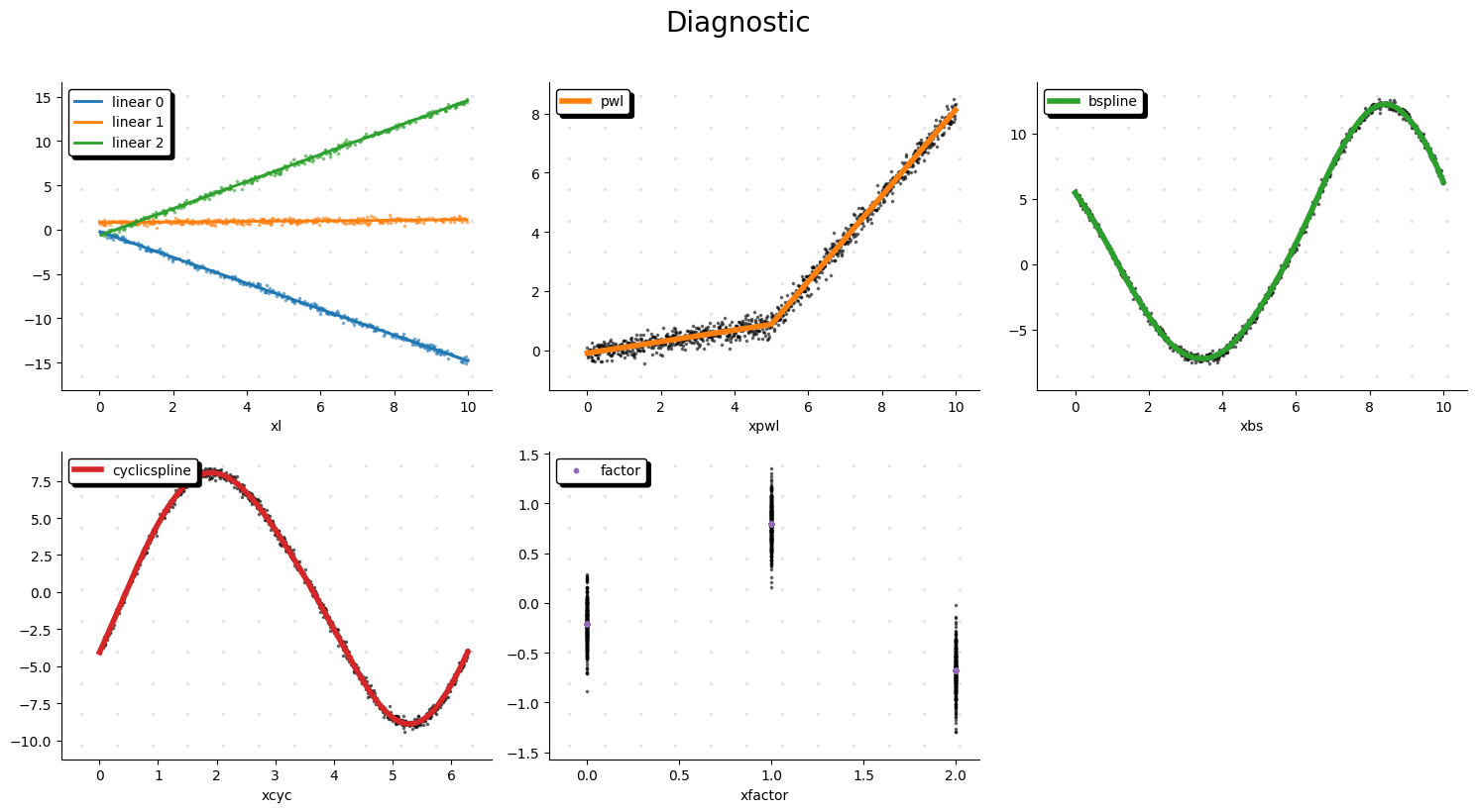
from lpspline import bs
from lpspline.constraints import Monotonic, Convex, Anchor, Concave

# -------------------------- Create demo dataset with wiggly target
np.random.seed(50)
N = 1000
x = np.linspace(-5, 5, N)
by = np.random.randint(0, 3, N)
y = (np.tanh(x)+1) + np.exp(-x/5) + np.sin(2*x)/2 +  np.random.randn(N)*0.05
df = pl.DataFrame({"x": x, 'by': by,"y": y})


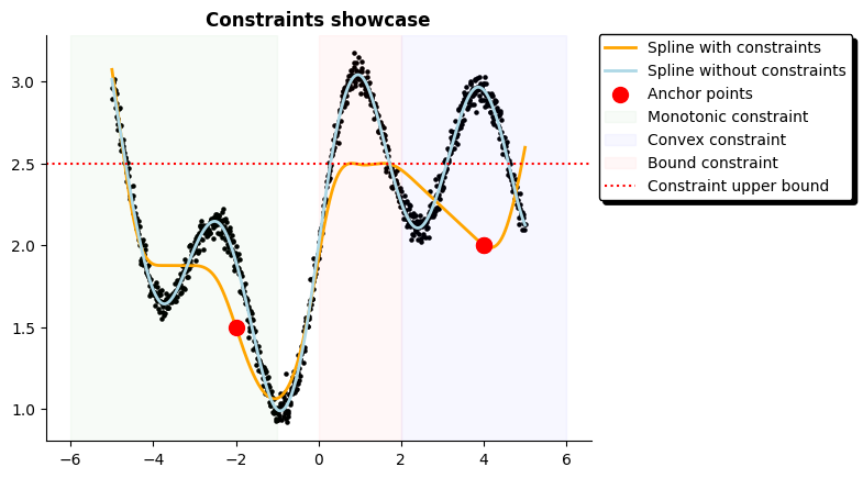
# -------------------------- Model with constraints
anchor_points = [(-2, 1.5), (4, 2)]
model = (
    # Try changing the spline using pwl or cs
    +bs("x", knots=np.linspace(-10, 10, 30), degree=3, tag='bs')
    .add_constraint(
        # Try changing the constraint here
        Convex(start=2, end = 10),
        Monotonic(decreasing=True, start=-10, end = -1),
        Anchor(*anchor_points),
        Bound(lower=None, upper=2.5, n=10, start=0, end=2)
    )
)


# -------------------------- Model without constraints for comparison
model_nocs = (
    +bs("x", knots=np.linspace(-10, 10, 30), degree=3, tag='bs')
)

model.fit(X=df, y=df['y'])
model_nocs.fit(X=df, y=df['y'])


# -------------------------- Cute plot to visualize result
plt.scatter(df['x'], df['y'], color='k', s=5)
plt.plot(df['x'], model.predict(df), color='orange', linewidth=2, label='Spline with constraints')
plt.plot(df['x'], model_nocs.predict(df), color='lightblue', linewidth=2, label='Spline without constraints')
for p in anchor_points:
    plt.scatter(*p, color='r', s=100, zorder=100)
plt.scatter(*p, color='r', s=100, zorder=100, label='Anchor points')

plt.axvspan(xmin=-6, xmax=-1, color='green', alpha=.03, label='Monotonic constraint')
plt.axvspan(xmin=2, xmax=6, color='blue', alpha=.03, label='Convex constraint')
pmp.legend(loc='ext side upper right')
pmp.remove_axis('top', 'right')
plt.title('Constraints showcase', fontweight='bold')

Link functions

import numpy as np
import polars as pl
import matplotlib.pyplot as plt
import pimpmyplot as pmp

from lpspline import l
from lpspline.link import Log, Exp

# ----------------- Demo dataset
N = 1000
X = pl.DataFrame({
    'x': np.linspace(1.,10, N)
})
y = pl.Series(np.log(X['x']) + np.random.randn(N)*0.1)

# ----------------- Model with log link
model = Exp(
    +l(term='x') # This is a linear term!
)
model.fit(X, y, summary=False)

# ----------------- Plot
plt.scatter(X['x'], y, color='r', alpha=.5, s=10, label='target')
plt.scatter(X['x'], model.predict(X), color='k', alpha=.5, s=10, label='model')
pmp.legend()
pmp.remove_axis('top', 'right')
pmp.bullet_grid()
plt.title('Link regression', fontweight='bold')