Quickstart#
Installation#
Install lpspline via pip directly from the command line:
pip install lpspline
Basic Usage#
LPSpline optimizes shape-constrained additive configurations utilizing convex methods (via CVXPY). It generates regression equations binding B-Splines, Linear blocks, or Categorical matrices smoothly.
For each spline type there is a dedicated class you can import
from lpspline import c, f, l, pwl, bs, cs
c: constantf: factorl: linearpwl: piecewise linearbs: B-splinecs: cyclic spline
LpRegressor#
The class LpRegressor is a sklearn-like interface to perform a regression with your data.
The easiest way to initialize an instance is to simply write down the formula.
from lpspline import c, f

mymodel = (
   l(term='x')
   + f(term='c')
)
term is the name of the column in the DataFrame X the spline is fitted on.
Tip
If your model consist in just one spline you can initialize the instance like so:
mymodel = +l(term='x')
You can still initialize the LpRegressor creating an instance in the classical way:
mymodel = LpRegressor(splines=[l(term='x'), f(term='c')])
Fit and predict#
LpRegressor is compatible with sklearn syntax. It works with polars DataFrames and Series.
import polars as pl
import numpy as np
from lpspline import c, f

X = pl.DataFrame({
   'x': np.linspace(0, 10, 100),
   'c': np.random.randint(0, 10, 100)
})
y = pl.Series(X['x'] + X['c'] + np.random.randn(100))

mymodel = l(term='x') + f(term='c')
mymodel.fit(X, y)
y_pred = mymodel.predict(X)
Summary#
When you fit the model a summary is printed to the console with all main informations:
spline type
term
applied constraints
applied penalties
number of parameters
========================================================================================================================
✨ Model Summary ✨
========================================================================================================================
Problem Status: ✅ optimal
------------------------------------------------------------------------------------------------------------------------
Spline Type          | Term         | Tag             | Constraints          | Penalties            | Params
------------------------------------------------------------------------------------------------------------------------
🟢 Linear            | x            | linearspline    | None                 | None                 | 2
🟢 Factor            | c            | factorspline    | None                 | None                 | 10
------------------------------------------------------------------------------------------------------------------------
📊 Total Parameters                                                                                 | 12
========================================================================================================================
Saving and Loading#
You can save your trained LpRegressor model to a file and load it back later. This is useful for persisting models or sharing them.
# Save the model
model.save("my_model.pkl")

# Load the model back
from lpspline import LpRegressor
loaded_model = LpRegressor.load("my_model.pkl")

# Use the loaded model for predictions
predictions = loaded_model.predict(X)
Note
The model is saved using pickle. When saving, the underlying optimization problem state is cleared to ensure the object is serializable. The loaded model is fully functional for predictions but cannot be further optimized without re-fitting.
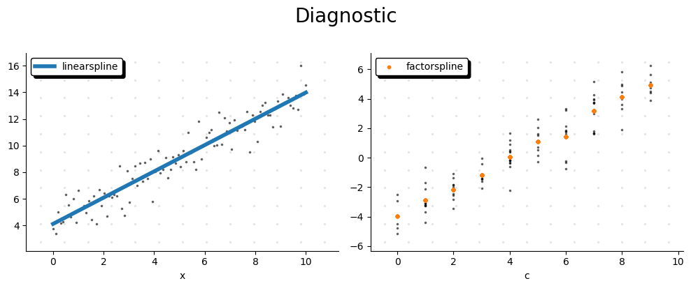
Diagnostics#
plot_diagnostic is a function that shows the diagnostic of the model.
It shows each fitted spline separately.
If you pass target to argument y: pl.Series it will be shown residuals relative to each spline as well.
In practice for each spline \(s_i\) it will be shown:
from lpspline import plot_diagnostic

plot_diagnostic(model=mymodel, X=X, y=y)